Problem Set 5 Answer Key
library(tidyverse)
library(lmSupport)
options(knitr.kable.NA = '')
1
reward <- read.csv("https://whlevine.hosted.uark.edu/psyc5143/ps4.csv", stringsAsFactors = TRUE)
group_means <- reward %>%
    group_by(COND) %>%
    summarise(M = mean(TRIALS))
grand_mean <- mean(reward$TRIALS)
The groups means are 8, 12, 24, 12 for the double-deprived, food-deprived, control, and water-deprived groups respectively, and the grand mean = 14; the latter is the same as the mean of the group means because the groups are of equal size.
The codes below are implemented in the script a bit more below.
contrast i: control = 3/4, others = -1/4
contrast ii: double-deprived = -2/3, single-deprived = 1/3
contrast iii: food-deprived = 1/2, water-deprived = -1/2
reward <- reward %>%
    mutate(x1 = ifelse(group == "b", 3/4, -1/4),
                 x2 = case_when(group == "b" ~ 0,
                                                 group == "c" ~ 1/3,
                                                 group == "d" ~ 1/3,
                                                 group == "e" ~ -2/3),
                 x3 = case_when(group == "b" ~ 0,
                                                 group == "c" ~ 1/2,
                                                 group == "d" ~ -1/2,
group == "e" ~ 0))- The contrasts all have a correlation of 0 with one another; so they’re orthogonal. I’ll also find tolerance for these after fitting the model. It will be 1 for each predictor.
cor(reward[4:6])## x1 x2 x3
## x1 1 0 0
## x2 0 1 0
## x3 0 0 1model1.contrasts <- lm(TRIALS ~ x1 + x2 + x3, reward)
params1 <- coef(model1.contrasts)The intercept of 14 is the mean of the group means. The slope of the first contrast is 13.3333, which equals the difference between the mean of the control group (24) and the mean of the three reward groups (i.e., (8 + 12 + 12) / 3 = 10.67). The slope of the second contrast is 13.3333, which equals the difference between the mean of the two singly-deprived groups (12) and the doubly-deprived group (8). And the slope of the last contrast is 4, which is the difference in the means of the two singly-deprived groups.
And look at the tolerances below!
1/car::vif(model1.contrasts) # 1/vif is tolerance## x1 x2 x3
## 1 1 1R2_model1.contrasts <- modelSummary(model1.contrasts)$r.squared\(R^2\) = 0.8955
modelEffectSizes(model1.contrasts)## lm(formula = TRIALS ~ x1 + x2 + x3, data = reward)
##
## Coefficients
## SSR df pEta-sqr dR-sqr
## (Intercept) 3920.00 1 0.9790 NA
## x1 666.67 1 0.8881 0.8292
## x2 53.33 1 0.3883 0.0663
## x3 0.00 1 0.0000 0.0000
##
## Sum of squared errors (SSE): 84.0
## Sum of squared total (SST): 804.0The three \(sr^2\) values do sum to \(R^2\). This is because the three contrasts fully code the differences among the three groups and they are orthogonal.
model_c <- lm(TRIALS ~ 1, reward)
SSE_C <- deviance(model_c)
SSE_A <- deviance(model1.contrasts)
SSR <- SSE_C - SSE_A
\(SSR\) = 720.
modelEffectSizes(model1.contrasts)The \(SSR\) values for x1, x2, and x3 are 666.67, 53.33, and 0, respectively. These add up to 720. Why? For the same reason that the \(\Delta R^2\) values add up to \(R^2\) for the whole model. See part i for more info.
- The figure below is a Venn diagram of the x1, x2, and x3 predictors, along with the outcome, Y (not drawn to scale, and not drawn to illustrate that x3 does not overlap with Y!). The three predictors don’t overlap because they are orthogonal. Regions a, b, and c represent the overlap of each predictor (i.e,. “explained” variance), respectively, and region e is the unexplained variance.
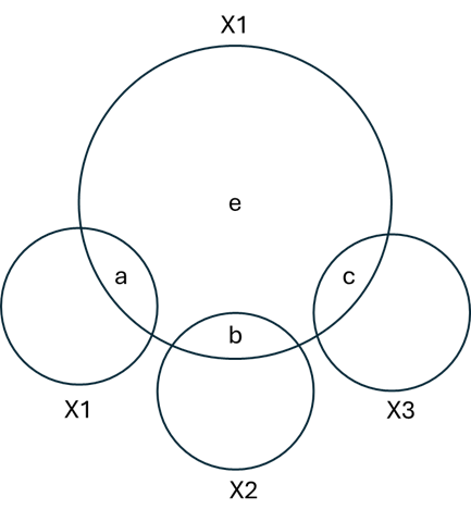
SSR for the whole model is a + b + c. SSR for x1 is a. SSR for x2 is b. SSR for x3 is c.
\(R^2\) for the whole model is \(\frac{a + b + c}{a + b + c + e}\)
\(\Delta R^2\) for x1 is \(\frac{a}{a + b + c + e}\).
\(\Delta R^2\) for x1 is \(\frac{b}{a + b + c + e}\).
\(\Delta R^2\) for x1 is \(\frac{c}{a + b + c + e}\).
The SSRs for individual predictors add up to SSR for the model, and the \(\Delta R^2\) values for the individual predictors add up to \(R^2\) for the model (because the SSRs and the \(\Delta R^2\) are just different representations of the same information).
- See below.
reward <- reward %>%
    mutate(dummy1 = ifelse(group == "c", 1, 0),
                 dummy2 = ifelse(group == "d", 1, 0),
                 dummy3 = ifelse(group == "e", 1, 0))
model1.dummy <- lm(TRIALS ~ dummy1 + dummy2 + dummy3, reward)
params1dummy <- coef(model1.dummy)The intercept is 24, which is the control group mean. Each of the other slopes is the deviation of the other group means from this value.
coef(lm(TRIALS ~ COND, reward))## (Intercept) CONDfood deprived CONDtwo per day control
## 8 4 16
## CONDwater deprived
## 4The intercept is the mean of the food and water deprived group and the slopes are deviations of other groups means from that value.
m&n)
reward <- reward %>%
    mutate(con4 = ifelse(group == "b", 3, -1),
                 con5 = case_when(group == "b" ~ 0,
                                                 group == "c" ~ 1,
                                                 group == "d" ~ 1,
                                                 group == "e" ~ -2),
                 con6 = case_when(group == "b" ~ 0,
                                                 group == "c" ~ 1,
                                                 group == "d" ~ -1,
                                                 group == "e" ~ 0))

modelSummary(lm(TRIALS ~ con4 + con5 + con6, reward))
The intercept is the same, but the slopes are fractions of what they were previously, 1/4 for contrast1, 1/3 for contrast2, and 1/2 for contrast4, although it’s hard to see that the latter is true because the slope is 0.
2
n2 <- read.csv("https://whlevine.hosted.uark.edu/psyc5143/threeGroups.csv")

n2groupMs <- n2 %>% group_by(group) %>% summarise(M = mean(memory))
n2grandM <- colMeans(n2groupMs[2])
The group means are 6, 12, 10 and the grand mean is 9.3333.
- I’ll go with control vs the two treatment groups and the treatment groups vs one another.
n2 <- n2 %>%
    mutate(con1 = ifelse(group == "control", -2/3, 1/3),
                 con2 = case_when(group == "control" ~ 0,
                                                 group == "rhyme" ~ 1/2,
                                                 group == "image" ~ -1/2))

model2 <- lm(memory ~ con1 + con2, n2)
params2 <- coef(model2)
SEs <- summary(model2)$coefficients[,2]
n2R2 <- summary(model2)$r.squared
The intercept and slopes are 9.3333, 5, -2, which are, respectively, the grand mean, the advantage for the two treatment group over the control, and the difference between the two treatment groups.
The SEs for the slopes are 1.4944, 1.7256. And \(R^2\) for the model = 0.3171.
model2weird <- lm(memory ~ con1, n2)
params2c <- coef(model2)
n2cSEs <- summary(model2weird)$coefficients[,2]
n2cR2 <- summary(model2weird)$r.squared
The intercept and slope are the same as they were for part b, although there is no slope for the difference in the two treatment groups.
The SE for the slope is 1.5036. And \(R^2\) for the model = 0.2831.
- The SE went up a bit and \(R^2\) went down. The reason is that what is considered residual error in the model in part c includes what was part of the explained variability of con2 in part b. More residual error means bigger SE and less explained variability. Look at the tables below and you’ll see that SSR for the model with only one contrast is exactly lower than the one with two contrast by the amount the SSR for the missing contrast. In this instance, SSR for the model with one contrast is 402; for the model with two contrasts it’s 422. The SSR for con2 in the model with two contrast is 20. This is not a coincidence.
modelEffectSizes(model2)
modelEffectSizes(model2weird)- See the code below. The model summary did not include con3. Why?
It’s entirely redundant with some combination of con1 and con2, revealed
by the error message that the
viffunction produces, “there are aliased coefficients in the model”. There is analiasfunction that reveals redundancy in a way that I’m still trying to interpret.
n2 <- n2 %>%
    mutate(con3 = case_when(group == "control" ~ 1/2,
                                                 group == "rhyme" ~ -1/2,
                                                 group == "image" ~ 0)) # control vs rhyme

model2e <- lm(memory ~ con1 + con2 + con3, n2)
coef(model2e) # con3 ignored!
## (Intercept) con1 con2 con3
## 9.333 5.000 -2.000 NA# car::vif(model2e) uncomment to run
# alias(model2e)3
n3 <- read.csv("https://whlevine.hosted.uark.edu/psyc5143/p3n3.csv")
is.factor(n3$groupF) # check!

# a, b, c
model3a <- lm(dv ~ groupF, n3); anova(model3a)
model3b <- lm(dv ~ group1, n3); anova(model3b)
model3c <- lm(dv ~ group2, n3); anova(model3c)
Here, F(2, 12) = 10.7 and SSE = 120.
Here, F(1, 13) = 0 and SSE = 333.
Here, F(1, 13) = 12 and SSE = 173.
The lowest SSE goes with the model in part a. One reason that this is the case is that this model has more parameters; numerator dfs provide critical information about the number of parameters the differ between Model C and Model A. Less obvious is that two linear relationships are being fit in this model, one for each of the underlying dummy codes, revealed by the R code below. In parts b and c, only one linear relationship is being evaluated. The consequence of the the latter is that this forces the use of the same slope to be used to accommodate the difference between two pairs of groups, which is very limiting.
Maybe the simplest way to say why group1 and group2 lead to higher values of SSE is to say that if you want to model differences between more than two groups, you’ll need at least two slopes to do so. Using one slope to do so is going to lead to suboptimal predictions.
- The models in parts b and c are treating group numbers as if the numbers having quantitative meaning. They don’t. They may as well be letters rather than numbers. THIS IS THE MORAL OF THE FABLE: IF YOU GET DATA WITH NUMBERS IDENTIFYING GROUPS, BE SURE TO TREAT THOSE NUMBERS AS LABELS RATHER THAN AS QUANTITATIVE VALUES.